A Survey of Differential-Algebraic Equations (1)

Motivation

We know that the general form of an ODE system is $u'(t) = f(u(t), p, t)$ where

• $f$ is called the derivative function or the right hand side of the ODE

• $u$ is called the dependent variable or the states.

• $p$ is the parameters.

• $t$ is the independent variable.

In a freshman differential equations course you will learn a bag of tricks to rearrange such equations to analytically solve them, i.e. to find the formula for $u(t)$. However, most of the ODEs are impossible to solve analytically, so in practice, we solve ODEs numerically. This means that we need to come up with some iterative procedure that approximates the function $u(t)$ for $t\in [a, b]\subseteq\mathbb R$ starting from $u(a)$.

The basic idea behind all numerical ODE solvers is to arrange terms in a particular way to truncate the Taylor series. For instance, let $h$ be the step size. The famous explicit Euler method is

Of course, there's a wide array of methods to solve ODEs, but they all originate from the idea of truncating Taylor series.

In engineering, the right hand side of the ODE often doesn't have an explicit formula. For instance, in a circuit, we know that the change of voltage is the current over the capacitance, i.e. $\frac{\mathop{}\!\mathrm{d} V}{\mathop{}\!\mathrm{d} t} = I(t) / C$. Also, the voltage and current follow the Kirchhoff laws, which form a system of linear equations. Hence, the governing equations of circuits naturally have both differential equations and algebraic equations.

We also want to compose different components together to build a larger model, and connection equations are algebraic relations among the state variables. It's possible to reduce algebraic equations away so that we are only left with explicit differential equations. However, this process is extremely time consuming and error-prone. Also, we lose the composability and the acausalness in the process. Hence, we want to use algorithms to automate the simplification and simulation of differential-algebraic equations (DAEs) to make modeling large scale simulation possible.

Numerical methods for DAEs

Like we hinted before, ODEs with algebraic relations among its states are DAEs. We can rephrase this as "differentiated states $u'(t)\in\mathbb R^n$ and states $u(t) \in\mathbb R^n$ form an implicit relation together with parameters $p\in\mathbb R^m$ and the independent variable $t\in\mathbb R$." Translating that into a formula gives

where $F: (\mathbb R^n, \mathbb R^n, \mathbb R^m, \mathbb R) \rightarrow \mathbb R^n$.

Similar to ODEs, we can truncate the Taylor series of $u(t)$ to solve the above system. The explicit Euler method becomes

Let's introduce $\hat{u}(t+h) \equiv u(t+h) + O(h^2)$ to denote the numerical solution to avoid visual clutter. As we already need to solve the implicit equations to approximate $u(t+h)$ using $\hat{u}(t+h)$, we can use the implicit Euler method to gain more stability

Numerically, we use Newton's method to solve potentially nonlinear equations by solving the best approximating linear equations (i.e. the Jacobian of the nonlinear function with respect to the unknowns) iteratively to refine an initial guess. By the chain rule, we have

The Newton iteration is then

where $\{\cdot\}^{[i]}$ denotes the iteration variable at the $i$-th iteration. Astute readers will notice that the Jacobian in Newton's method is a matrix pencil of the form $J(\lambda) = A + \lambda B$. We know that Newton's method only makes sense when there exists a $\lambda \in \mathbb R$ (a suitable step size) such that $\det(J(\lambda)) \ne 0$ (J is invertible), or in other words, the matrix pencil is regular.

Numerically motivated characterizations of DAEs

A natural question is: how can we relate DAEs to ODEs? Notice that $F$ is 0 for all $t$, so the derivative of $F$ with respect to time also gives a new set of equations, so do any higher order time derivatives of $F$, i.e.

We need a way of knowing when differentiating $F$ does not add new "information" into the system. First, let's develop a characterization on the variables. Let $z$ be the set of the highest order derivative variables, and let $\lambda$ contain the rest of the variables. Note that $z$ and $\lambda$ must be disjoint. Therefore, DAEs can then be written as

Differentiating the above equation gives us

Note that $z'$ contains all the new terms generated by the differentiation, as it contains variables with higher order derivatives than before. Rearranging terms, we get

When $\hat{F}_z$ is invertible, we can use old terms to explicitly solve for $z'$, so we don't generate genuinely new equations. Therefore, we only add new equations to the system if and only if $\hat{F}_z$ is singular. It's wasteful to differentiate the entire system until the matrix is invertible; we can differentiate a minimal subset of equations to make $\hat{F}_z$ fully ranked.

Also, note that the above equation can be converted to an ODE if $\hat{F}_z$ is invertible. We can characterize DAEs by the number of differentiations needed to convert it into an ODE, and we call this property the index of a DAE. In particular, when the Jacobian matrix $\hat{F}_z$ is invertible, the system is index 1. Here, we note that the numerical significance of an index 1 DAE system is that, we can initialize and solve the system easily with Newton's method because all the "latent" equations appear in the system, or in other words, $\hat{F}_z$ is invertible, so all the constraining variables can be solved from the differential variables.

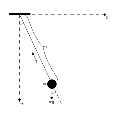
Now, let's translate the theory into a concrete example. The equations of motion of the pendulum system in Cartesian coordinate $(x, y)$ are

where $T$ is the tension from the string, $g$ is the gravitational acceleration, $r$ is the length of the string, and we assume the mass of the object is 1. Physically, we know that $T$ must be uniquely determined from $x''$ and $y''$. However, computing $T$ is not obvious given the above equations. Let's use the mathematical tools that we defined earlier to analyze this system.

The highest order derivative terms are $z = (x'', y'', T)$. Note that $T$ is one of the highest order derivative terms because no derivative of $T$ appears in the system. The exact rank of $\hat{F}_z\in \mathbb R^{n\times n}$ is too difficult to compute because it's time-varying. In practice, we use the sparsity pattern or the structure of the Jacobian to determine its structural rank — a weak version of the numerical rank. We can use a bipartite graph to represent the sparsity pattern. We define the structural rank as the maximum cardinality of the bipartite matching. If we assume that no cancellations among the non-zero entries are possible, then the structural rank is exactly the numerical rank.

The structure of $\hat{F}_z$ from the pendulum system is

which is clearly singular. Hence, we cannot use Newton's method to compute $T$ from given $x''$ and $y''$. Since only the last row of the matrix is problematic, we just need to use differentiations to introduce $x'', y''$, or $T$ into the last equation to make the Jacobian structurally fully ranked. Differentiating the last equation twice, we get

Now, the structure of $\hat{F}_z$ is

which has full structural rank. Note that we can simplify the differentiated equation by substituting the differential equations into it, which gives us

The resulting system is

We can use the initial condition of $x$, $x'$, $y$, and $y'$ to uniquely determine the initial condition of the tension $T$, because $\hat{F}_z$ is invertible. This also means that the resulting system is an index 1 DAE, and the original pendulum system is index 3, since we differentiated the last equation twice. Lastly, as an exercise, we can get the underlying ODE by differentiating the last equation one more time

which implies

Hence, the ODE system is then